DDIA Chapter 4 Notes: Storage and Retrieval

At the most fundamental level, a database does two things: it stores data when you give it to it, and it gives the data back when you ask for it. This chapter dives into how databases handle storage and retrieval internally, focusing on the distinct architectural differences between operational (OLTP) and analytical (OLAP) workloads.
The Chinese translated edition of the book:

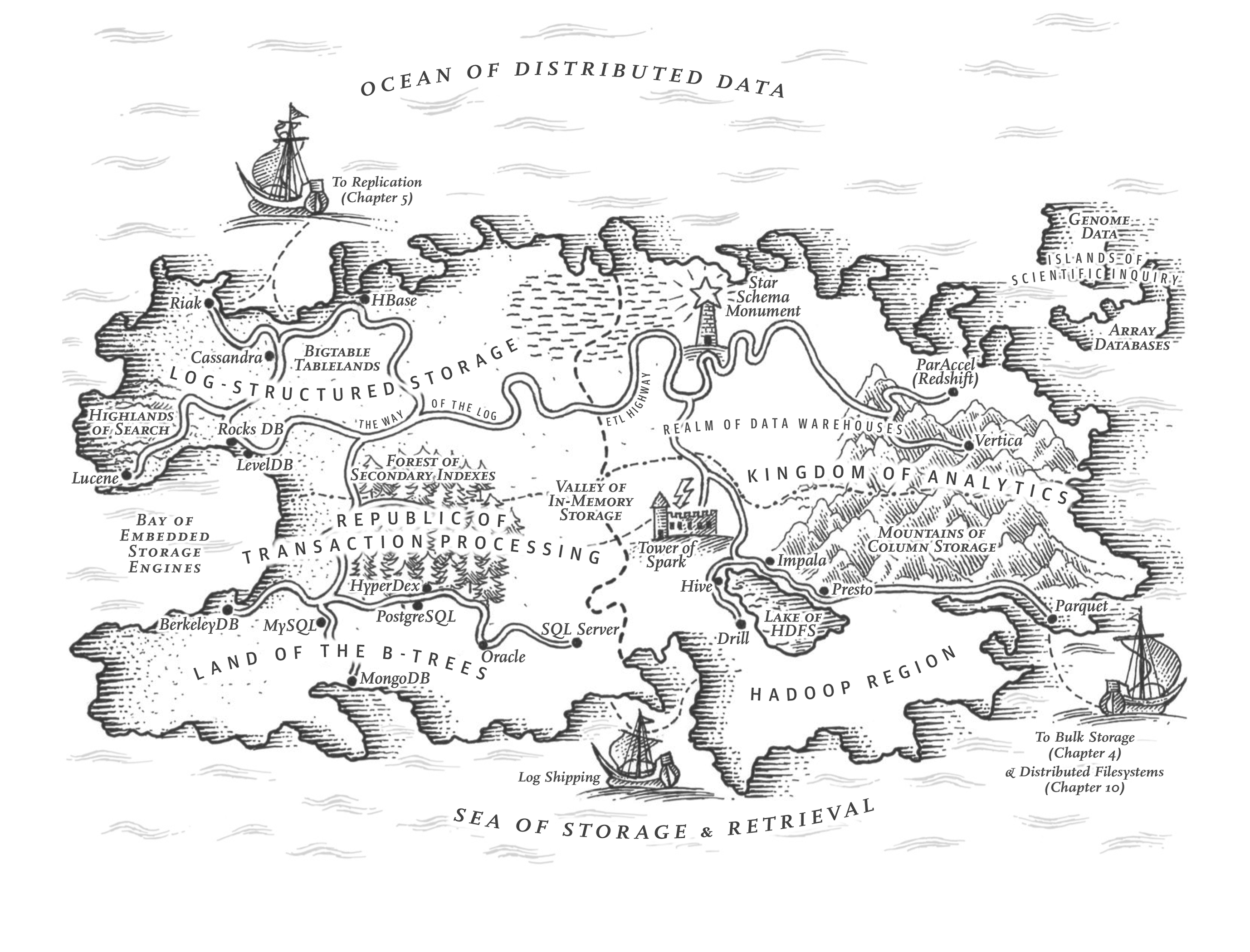
If you are interested in the foundational concepts of data systems, you can also check out my notes on Chapter 2:
 Joanne
Table of Contents
OLTP Storage and Indexing
To efficiently find the value for a particular key in a database, we need a data structure called an index. An index is an additional structure derived from the primary data. While well-chosen indexes speed up read queries, every index slows down writes because it must be updated whenever data is written.
(為了高效檢索資料,資料庫需要建立索引。索引能加速讀取,但會因為寫入時的同步更新而拖慢寫入效能,這是在儲存系統設計中必須權衡的關鍵。)
Log-Structured Storage
A fundamental way to store data is using an append-only log, which provides efficient $O(1)$ writes. However, reading from a plain log is $O(N)$ because the database must scan the entire file to find a specific key.
To optimize reads, systems maintain an in-memory hash map tracking the exact byte offset of each key's latest value. Keeping this index in memory is crucial because hash map lookups require jumping to unpredictable locations, which is extremely slow on disks but fast in memory. Furthermore, on-disk hash maps are expensive to resize and are inefficient for range queries because hashing destroys the natural sorting order, placing sequential keys (like ID 1 and ID 2) in completely different locations.
(僅追加日誌寫入極快但讀取慢。系統雖透過記憶體雜湊表來加速讀取,但其硬碟隨機存取效能差,且不利於範圍查詢。)
SSTable File Format
To address the limitations of hash indexes, the Sorted String Table (SSTable) format requires key-value pairs to be strictly sorted by key, and each key appears only once per file.
This sorting introduces two major advantages:
- Efficient Range Queries: They leverage sequential disk I/O, significantly speeding up reads.
- Sparse In-Memory Index: The system only needs to store memory pointers for a subset of keys (acting as signposts). For any target key, it simply jumps to the closest preceding key and scans a short distance.
(SSTable 透過嚴格按鍵排序,不僅大幅提升範圍查詢的效率,還能以稀疏索引有效降低記憶體負擔。)
Constructing and Merging SSTables
Writing randomly to a sorted file on disk is inherently slow. Log-Structured Merge-Trees (LSM-trees) solve this using a multi-step process:
- Memtable: Incoming data is written to an in-memory balanced tree, naturally maintaining sorted order.
- WAL (Write-Ahead Log): To prevent data loss on crash, every write is simultaneously appended to a durable, unsorted log on disk.
- SSTable Flush: Once the Memtable reaches a threshold, it is flushed sequentially to disk as an immutable segment.
- Tombstones: Deletions write a special marker. Background compaction later merges segments and discards the invalid values safely.
(LSM 樹將資料先寫入記憶體 (Memtable) 並配合 WAL 防範斷電遺失,滿載後再循序寫成 SSTable。資料刪除則依賴「墓碑」標記,待背景壓實時再徹底清除。)
Bloom Filters
Looking up a non-existent key in an LSM-tree can be expensive, as the engine must check the Memtable and scan through multiple on-disk segments from newest to oldest. To mitigate this, databases employ Bloom filters—a highly memory-efficient bit array that relies on probability.
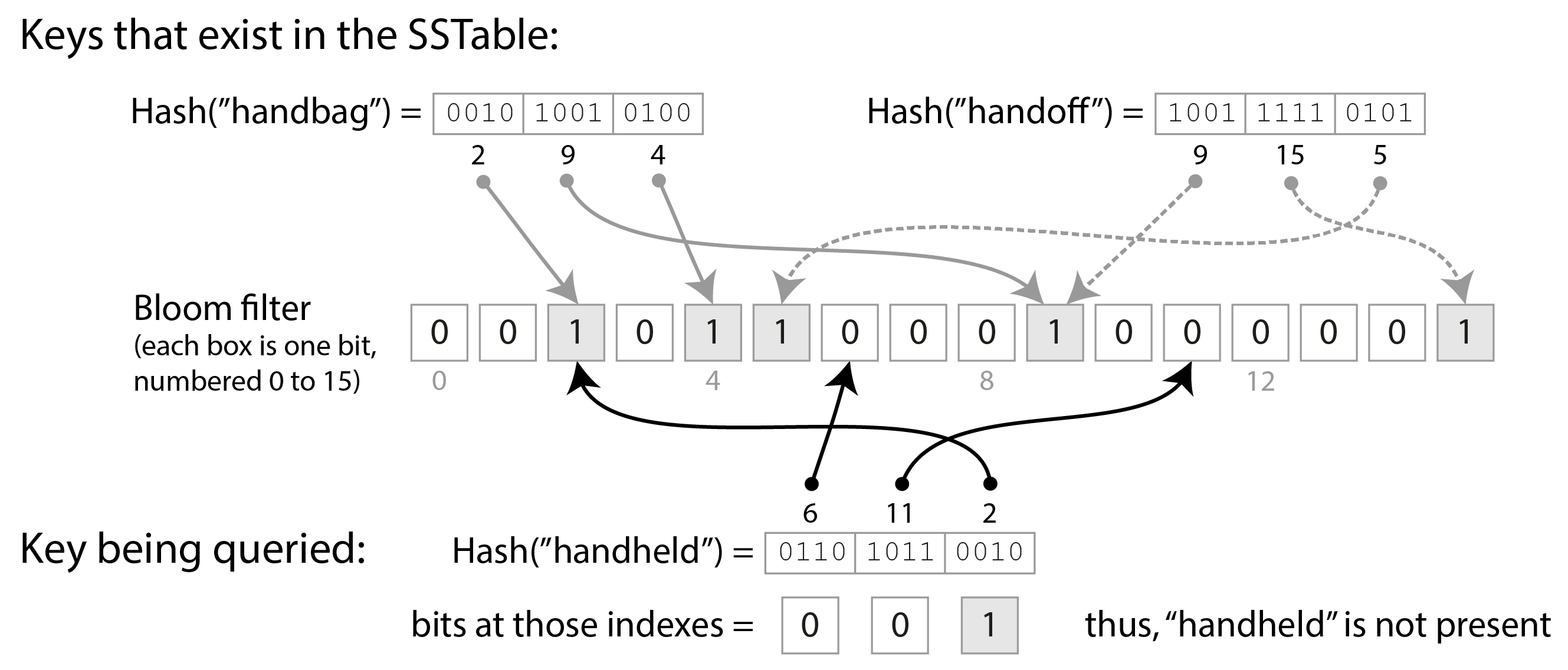
The filter operates through a straightforward mechanism:
- Initialization: A fixed-size bit array is created, with all bits initially set to
0. - Insertion: When a key is written to a segment, it is processed by multiple hash functions. Each function generates an index, and the corresponding bits in the array are updated to
1. - Querying: To search for a key, the engine hashes it using the exact same functions. If any of the resulting indices contain a
0, the key definitively does not exist in that segment, allowing the engine to safely skip the file (zero false negatives). If all indices contain a1, the key is probably present (a potential false positive caused by hash collisions from other keys), and the engine proceeds with a disk read.
While it may occasionally yield a false positive, the Bloom filter effectively eliminates the vast majority of unnecessary disk reads, optimizing query performance with minimal memory overhead.
(為避免 LSM 樹在查詢無效資料時耗費硬碟 I/O,系統採用布隆過濾器:寫入時以雜湊標記位元,查詢時若遇 0 即保證資料絕對不存在。雖偶有誤判,但它能以極小記憶體擋下絕大多數的無效讀取。)
Compaction Strategies
Compaction is essential for merging sorted files and cleaning up garbage (like tombstones), but different strategies offer distinct trade-offs:
- Size-tiered compaction: Merges files of similar sizes. This approach maximizes write throughput because the engine simply combines files without strictly sorting or partitioning their key ranges. However, it results in overlapping key ranges across multiple large files (slowing down reads) and requires a significant amount of temporary disk space to hold the newly merged file before the old ones can be deleted.
- Leveled compaction: Organizes files into distinct levels with fixed sizes. Within a level, key ranges never overlap. This gradual approach requires more upfront sorting work (resulting in slightly lower write throughput), but it guarantees highly efficient reads since a key can only reside in one specific file per level. Additionally, because it merges only a few small files at a time, it avoids sudden storage spikes and maintains a predictable, minimal temporary disk space overhead.
To summarize the key differences between the two strategies:
| Feature | Size-Tiered Compaction | Leveled Compaction |
|---|---|---|
| Core Logic | Merges files based on size, resulting in increasingly larger files. | Merges files incrementally into the next level based on precise key ranges; individual file sizes remain fixed. |
| Read Performance | Slower (requires scanning multiple large files with overlapping key ranges). | Extremely fast (non-overlapping ranges allow precise targeting of a single small file). |
| Write Performance | Extremely fast (simple merge logic imposes minimal overhead on incoming writes). | Slower (merging requires strict key range comparisons and sorting). |
| Disk Space Overhead | Very high (requires massive temporary buffer space to merge huge files). | Minimal and stable (merges only a few small files at a time in the background). |
(分層壓實合併速度快,但易產生範圍重疊與空間波動;分級壓實讀取極快且空間消耗穩定,但寫入成本略高。)
B-Trees
Introduced in 1970, B-trees remain the standard index implementation in almost all relational databases. Unlike log-structured storage (LSM-trees), which break data into variable-size segments and append them sequentially, B-trees break the database down into fixed-size blocks or pages (traditionally 4 KiB to 16 KiB) that closely align with the underlying hardware architecture. This design relies on in-place updates: when a record changes, the B-tree locates the exact page on disk and overwrites it, rather than appending a new record to the end of a file.
To summarize the fundamental architectural differences between these two storage models:
| Feature | Log-Structured Storage (e.g., LSM-Tree) | B-Tree |
|---|---|---|
| Space Management | Variable-size segments (SSTables). | Fixed-size blocks or pages. |
| Update Mechanism | Append-only: Sequentially writes new data to the end of a file, leaving old data untouched. | In-place update: Locates the specific page on disk and overwrites it directly. |
| Primary Advantage | Exceptionally fast write performance (no seeking required, just appending). | Predictable, stable read performance and minimal generation of obsolete data. |
(B 樹將資料劃分為固定頁面以契合硬碟特性,並採就地覆寫。相較於 LSM 樹的僅追加機制,B 樹能提供更穩定的讀取效能,且無須龐大的背景清理。)
Navigating the Tree and the Branching Factor
Each page in a B-tree can be identified using an address or byte offset, allowing one page to refer to another, similar to a pointer. Traversing a B-tree always starts from a single root page and navigates down through interior pages containing boundary keys, eventually reaching a leaf page that contains the actual data or a reference to it.
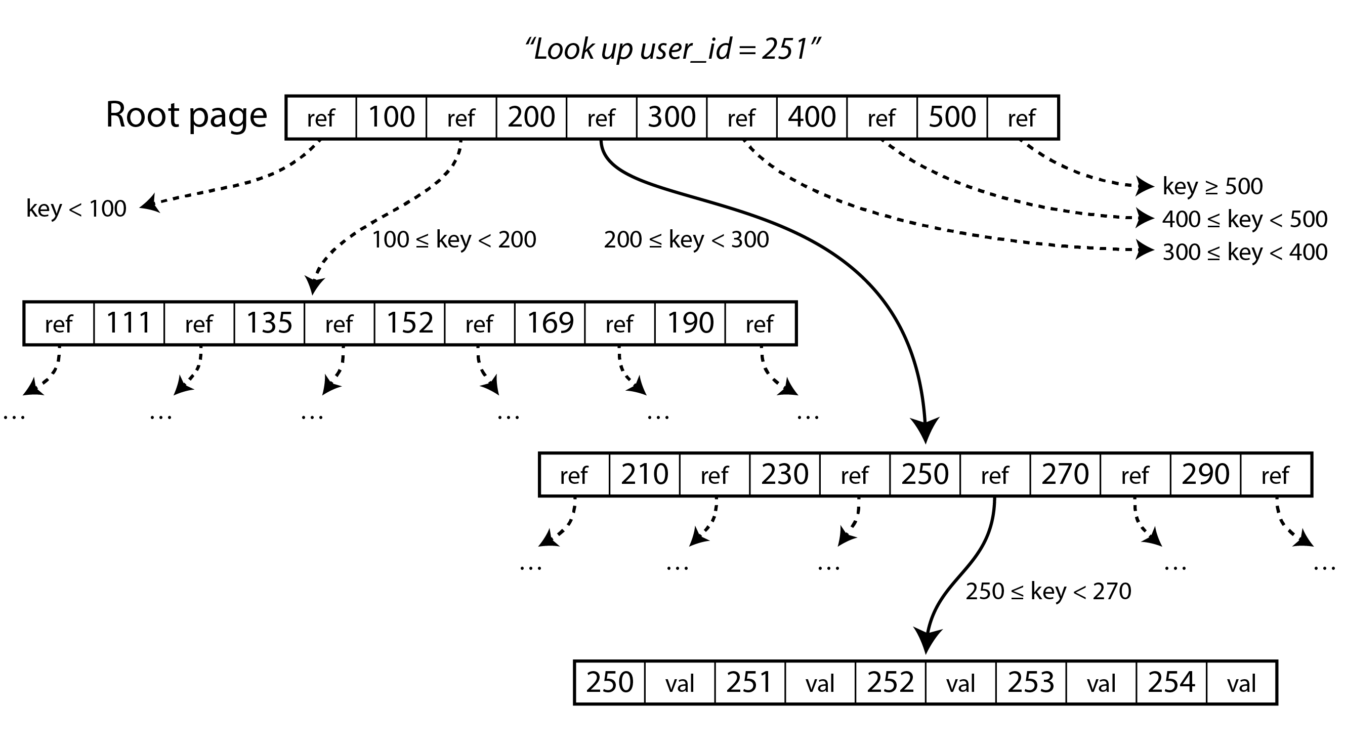
The number of references to child pages within a single page is called the branching factor. Because page references and keys are relatively small compared to the page size (e.g., 16 KiB), the branching factor is typically several hundred (e.g., 500). This enables exponential capacity growth: a four-level tree with a branching factor of 500 can hold up to 250 TB of data. Consequently, finding a specific record out of billions requires following only three or four page references, resulting in a highly predictable $O(\log n)$ read performance.
(B 樹因分支因子極大而呈現矮胖結構,即使資料量龐大,也只需少數幾次硬碟讀取即可精準定位,查詢效能非常穩定。)
Making B-Trees Reliable: Memory Buffering and the WAL
Overwriting a page on disk is a risky operation. If a database crashes mid-overwrite (e.g., only writing 8 KiB of a 16 KiB page), it results in a partially updated, corrupted block known as a "torn page." Furthermore, performing random disk I/O for every single update significantly degrades performance.
To address both issues, B-tree implementations buffer modified pages in volatile memory (often called the Buffer Pool) to batch write operations. To prevent data loss from a sudden power failure, they rely heavily on a Write-Ahead Log (WAL). Every modification must be quickly appended to this durable, sequential log before the in-memory pages are altered. In the event of a crash, the WAL provides the exact instructions needed to repair torn pages and restore the tree index to a fully consistent state.
(B 樹透過記憶體緩衝批次處理分頁更新,並強烈依賴預寫式日誌 (WAL) 防範當機導致的撕裂寫入,以確保資料一致性。)
The Shared Strategy with LSM-Trees
Interestingly, log-structured engines (LSM-trees) face the exact same physical disk limitations and adopt an identical overarching strategy: they buffer incoming writes in memory (the Memtable) for performance, and append them to a WAL for crash recovery.
While the "Memory Buffer + WAL" design pattern is universal across modern databases, the underlying storage philosophy dictates a subtle difference in how the WAL is managed:
- In B-Trees (Structural Rescuer): Because B-trees perform in-place updates, the WAL is strictly necessary to recover from partial overwrites and repair corrupted tree structures.
- In LSM-Trees (Temporary Safeguard): Because LSM-trees are append-only, there are no in-place overwrites to corrupt. The WAL acts solely as a backup for the volatile Memtable. Once the Memtable is safely flushed to disk as an immutable SSTable, that corresponding WAL segment becomes obsolete and is safely discarded.
(兩者皆依賴「記憶體緩衝+WAL」。差異在於 B 樹需要 WAL 來修復就地覆寫的結構損壞,而 LSM 樹的 WAL 僅為暫時備份,寫出檔案後即可丟棄。)
B-Tree Variants
Over decades of optimization, several variants have emerged to address specific limitations (most notably the B+ Tree architecture, which is the modern standard):
- Copy-on-Write: Instead of overwriting pages and maintaining a WAL, some databases write modified pages to a new, empty location and create new versions of parent pages pointing to it. This inherently prevents partial overwrites and significantly aids concurrency control.
- Key Abbreviation: Interior pages do not need to store entire keys; they only need enough information to act as boundaries between key ranges. This saves space, significantly increasing the branching factor and keeping the tree shallower.
- Sequential Physical Layout: Some implementations attempt to lay out leaf pages sequentially on the physical disk to optimize large range queries, though this is difficult to maintain as the tree grows and requires periodic defragmentation.
- Sibling Pointers (B+ Tree): Leaf pages often include direct references to their left and right siblings. This allows the database to scan sequentially across a range of keys without repeatedly jumping back up to parent pages.
(B 樹發展出多種優化變體,例如:寫時複製提升併發性、縮寫鍵降低樹高,或透過相鄰指標 (B+ 樹) 加速範圍查詢。)
Comparing B-Trees and LSM-Trees
As a rule of thumb, LSM-trees are typically faster for writes, whereas B-trees are faster for reads.
Read Performance and Latency Predictability
- Point Queries: Reads in B-trees are predictably fast, as traversing the index requires following only a few page references. LSM-trees might need to check multiple SSTables, making point queries slightly slower, though Bloom filters help mitigate this by filtering out unnecessary disk reads.
- Range Queries: The performance gap widens significantly during range queries. B-trees (specifically B+ trees) excel here by directly scanning horizontally across linked leaf pages. LSM-trees struggle because Bloom filters cannot evaluate ranges, forcing the engine to scan and merge multiple files simultaneously on the fly.
- Latency Predictability: While LSM-trees offer exceptional write throughput, sustained heavy writes can cause background compaction to fall behind. To prevent memory exhaustion, the engine triggers backpressure, temporarily pausing requests and causing sudden latency spikes (compaction stalls). B-trees avoid these massive background merges, providing much more stable and predictable performance overall.
(一般而言,B 樹在點查詢與範圍查詢皆提供穩定的高效能;LSM 樹則寫入極快,但範圍查詢較弱,且在高壓寫入時易因壓實作業不及而產生延遲峰值。)
Sequential and Random Writes
B-trees update pages in place, translating scattered application updates into heavy random disk writes. In contrast, LSM-trees decouple logical sorting from physical location by buffering writes in a Memtable and flushing them as large, contiguous segments. This effectively converts random application updates into highly efficient sequential writes.
While SSDs lack moving mechanical parts, they still strongly favor sequential writes due to their physical constraints. SSDs write data in small pages but can only erase data in much larger blocks, and they cannot overwrite data in place. B-tree's random writes heavily fragment these blocks with a mix of valid and invalid data, forcing the SSD controller to constantly relocate valid pages before erasing—a costly process known as Garbage Collection (GC).
By writing massive sequential chunks, LSM-trees avoid this fragmentation. When older SSTables become obsolete, the SSD can often erase entire blocks at once without expensive page-relocation operations. Consequently, LSM-trees sustain significantly higher write throughput and induce far less wear (write amplification) on modern drives.
(B 樹的就地覆寫易產生碎片化,加重 SSD 的垃圾回收負擔。LSM 樹則透過批次連續寫入,有效降低硬碟磨損並提升吞吐量。)
Write Amplification
A single application write request often translates to multiple physical disk writes over its lifetime—a phenomenon called write amplification. High write amplification acts as a multiplier on disk wear and limits the maximum throughput a database can handle.
In a B-tree, modifying a 4-byte record requires rewriting the entire 4 KiB (or 16 KiB) page to disk, plus the WAL entry. In an LSM-tree, data is also written multiple times: first to the WAL, then flushed to an SSTable, and rewritten repeatedly during background compactions. Despite this, LSM-trees typically exhibit lower write amplification than B-trees because they write compressed, dense blocks sequentially, rather than rewriting largely unchanged, fragmented pages.
However, LSM compaction can still cause severe write amplification if the values (data payloads) are large, as massive amounts of data are repeatedly rewritten during merges. To mitigate this, some LSM engines implement key-value separation (e.g., WiscKey). The large values are written once to a separate, append-only "value log," while the LSM-tree only stores and compacts the small keys and pointers. This prevents large payloads from participating in costly compactions, significantly reducing write amplification.
(寫入放大指實際寫入量大於請求量。B 樹因覆寫整頁產生放大,LSM 樹因反覆壓實產生。若負載極大,LSM 樹可透過鍵值分離技術減輕 I/O 負擔。)
Disk Space Usage and Immutability
B-trees inherently suffer from fragmentation due to in-place updates and required buffer space (fill factors). They often require expensive background operations (like VACUUM) to defragment and return unused space to the OS. In contrast, LSM-trees generate significantly smaller files. Because SSTables are strictly immutable and written sequentially, the engine packs data at 100% density. Furthermore, this physical sorting allows for highly aggressive prefix compression.
Immutability, however, is a double-edged sword. For deletions, LSM-trees must write "tombstones" that slowly propagate through compactions before data is physically erased—a challenge for strict privacy regulations (often mitigated by cryptographic erasure).
Conversely, immutability makes taking instantaneous, zero-copy backups trivial. A snapshot simply records the active SSTable filenames, requiring virtually no disk I/O. Taking a similar snapshot in a B-tree is vastly more complex, often requiring Copy-on-Write mechanisms to prevent historical pages from being overwritten.
(B 樹易產生空間碎片;LSM 樹因連續寫入能達成極高壓縮率與瞬間零拷貝快照,但處理資料刪除時須等待背景壓實完成。)
Multi-column and Secondary Indexes
To query data efficiently, databases utilize different types of indexes. The most fundamental is the primary key index, but secondary indexes are essential for querying data by attributes other than the primary identifier. We can distinguish them by what they physically store:
| Primary Index | Secondary Index | |
|---|---|---|
| What the Key Stores |
Unique Primary Key (e.g., ID 101)
|
Search condition (e.g., [email protected])
|
| What the Value Stores | The complete row data (e.g., Name, Email, Password). |
The corresponding Primary Key ID (e.g., 101).
|
| Retrieval Logic | Look up the key to directly retrieve the full record. | Look up the key to get the ID, then query the Primary Index with that ID to retrieve the full record. |
(資料庫的索引主要分為兩種:主鍵索引透過唯一 ID 直接取得完整資料;次要索引則是透過搜尋條件先找到對應的 ID,再「回表」去主鍵索引撈出完整資料。)
Handling Non-Unique Keys in Secondary Indexes
Secondary index keys (e.g., "John") are rarely unique, yet underlying engines (B-trees, LSM-trees) rely on unique keys to sort and navigate efficiently. Databases resolve this using two primary methods:
- List of Identifiers: The index key maps to an array of matching primary IDs (e.g.,
Key="John" -> Value=[ID_1, ID_2]). While common in full-text search, modifying a single ID within a massive list requires rewriting the entire array, creating a significant I/O bottleneck. - Appending the Primary Key: The engine concatenates the search term with the primary ID to create a globally unique key (e.g.,
Key="John_001"). Because underlying trees keep keys strictly sorted, all "John" entries sit contiguously on disk. The database can retrieve them all via a highly efficient prefix scan, reading sequentially until the prefix changes.
(次要索引常遇鍵值重複的問題。常見解法為存入 ID 陣列,或將主鍵附加於搜尋鍵後創造唯一複合鍵,再利用前綴掃描快速檢索。)
Storing Values in the Index
How does an index deliver the actual data once a key is found? Databases generally use three architectural approaches:
- Clustered Index: Stores the complete row data directly within the index itself (e.g., MySQL InnoDB's primary key). Finding the key instantly yields the full record.
- Heap Files and References: Stores a pointer to the data rather than the full row. This pointer can be a primary key ID requiring a second lookup in the clustered index (MySQL), or a direct physical disk coordinate pointing to an entirely separate, unordered "heap file" (PostgreSQL).
- Covering Index: A performance optimization that stores copies of frequently queried columns alongside the secondary key. If a query only needs those specific columns, it bypasses the expensive secondary lookup, trading disk space and write speed for significantly faster reads.
(存放真實資料有三種方式:聚簇索引直接存放完整資料;次要索引存指標(回查主鍵或指向堆檔案);覆蓋索引則複製常用欄位以空間換取時間。)
In-Memory Storage
As RAM becomes cheaper, keeping entire datasets in memory becomes viable. In-memory databases are fast not primarily because they avoid disk reads (the OS caches disk blocks anyway), but because they eliminate the CPU overhead of encoding memory data structures into formats suitable for disk storage.
Specifically, operating entirely in memory eliminates several costly disk-centric operations:
- Serialization/Deserialization: Bypassing the need to constantly encode CPU-friendly data structures into compact byte arrays for disk storage, and vice versa.
- Buffer Pool Management: Removing the logic required to track, fetch, and evict pages between RAM and disk.
- Storage Maintenance: Eliminating the background I/O work of B-tree page splits or LSM-tree compactions.
- Complex Locking: Reducing the heavy concurrency control mechanisms originally designed to manage queues for slow disk I/O.
By stripping away these overheads, in-memory engines can achieve maximum execution speed, using disks only for append-only durability logs rather than active reading and writing.
(全記憶體資料庫的極速效能,源自於徹底省去了迎合硬碟產生的 CPU 運算開銷,如序列化、緩衝池管理及複雜的鎖定機制。)
Analytic Data Storage
While OLTP systems manage transactions, data warehouses handle complex read-only analytic queries (OLAP) scanning millions of rows.
Cloud Data Warehouses and the Open Lakehouse
Modern cloud data warehouses decouple query computation from the storage layer. Data is durably stored in scalable, low-cost object storage (like Amazon S3), while stateless compute resources are provisioned on demand. This allows organizations to scale storage and compute independently.
Beyond basic decoupling, the modern Open Data Lakehouse deconstructs the traditional, monolithic database into four interchangeable components built on open standards:
- Query Engine (e.g., Trino, Spark): The stateless compute layer responsible for executing queries and processing data.
- Storage Format (e.g., Parquet): Open file formats on disk. This prevents vendor lock-in, allowing any compatible tool to read data directly from cloud storage.
- Table Format (e.g., Apache Iceberg): Dynamic manifests that track which immutable files constitute a table, enabling ACID transactions and "time travel."
- Data Catalog (e.g., Snowflake Polaris, Unity Catalog): A centralized metadata registry allowing multiple disparate query engines to discover and share the exact same underlying data.
To summarize this architectural paradigm shift:
| Feature | Traditional Monolithic Database | Modern Open Lakehouse |
|---|---|---|
| Data Storage | Proprietary formats readable only by the specific engine. | Open file formats (e.g., Parquet) on cloud object storage. |
| Data Access | Must pass through the database's specific connection layer. | Direct access to cloud files via standard protocols. |
| Tooling | Locked into a single vendor's ecosystem. | Agnostic; shared seamlessly across Spark, Trino, Python, and AI tools. |
| Ecosystem | Closed (swapping engines requires massive data migration). | Open (compute engines can be swapped freely without moving data). |
(現代雲端資料倉儲將運算與儲存解耦以達成獨立擴展。進階的開放式資料湖架構進一步將系統拆分為查詢引擎、儲存格式、表格式與資料目錄四個開源模組,藉此避免廠商綁定,允許不同工具直接共享同一份底層資料。)
Column-Oriented Storage
Relational OLTP databases use row-oriented storage. If a query only needs 3 columns out of 100, row-oriented storage still loads the entire row. Column-oriented storage stores all values of each column together. Queries only parse the exact columns they need, significantly reducing disk I/O.
Column Compression
Column-oriented storage is highly amenable to compression. Because data within a single column is of the same type and often sorted (e.g., by date or product ID), repetitive values frequently cluster together (e.g., 69, 69, 69, 74). Storing these consecutive values as full integers is highly inefficient.
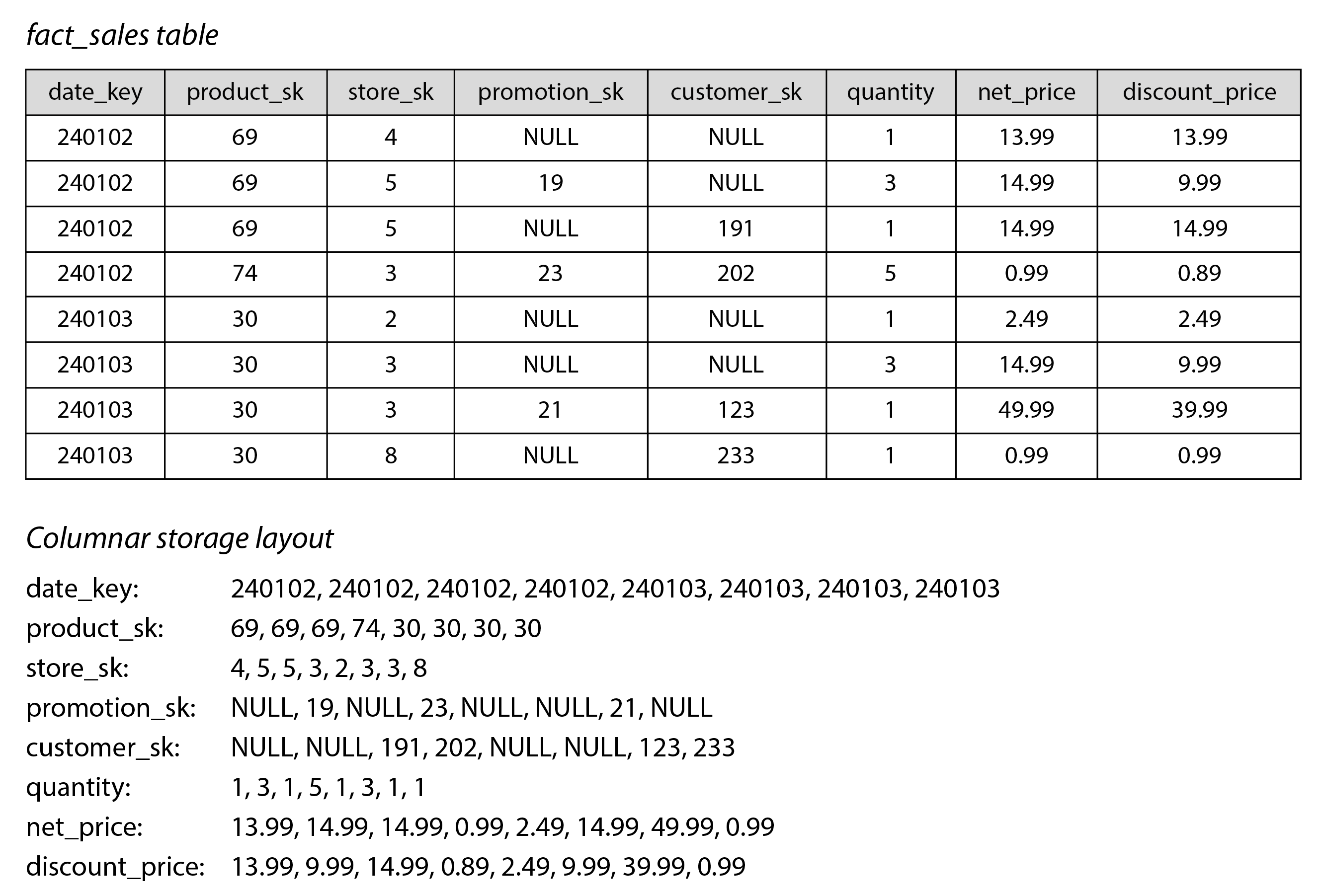
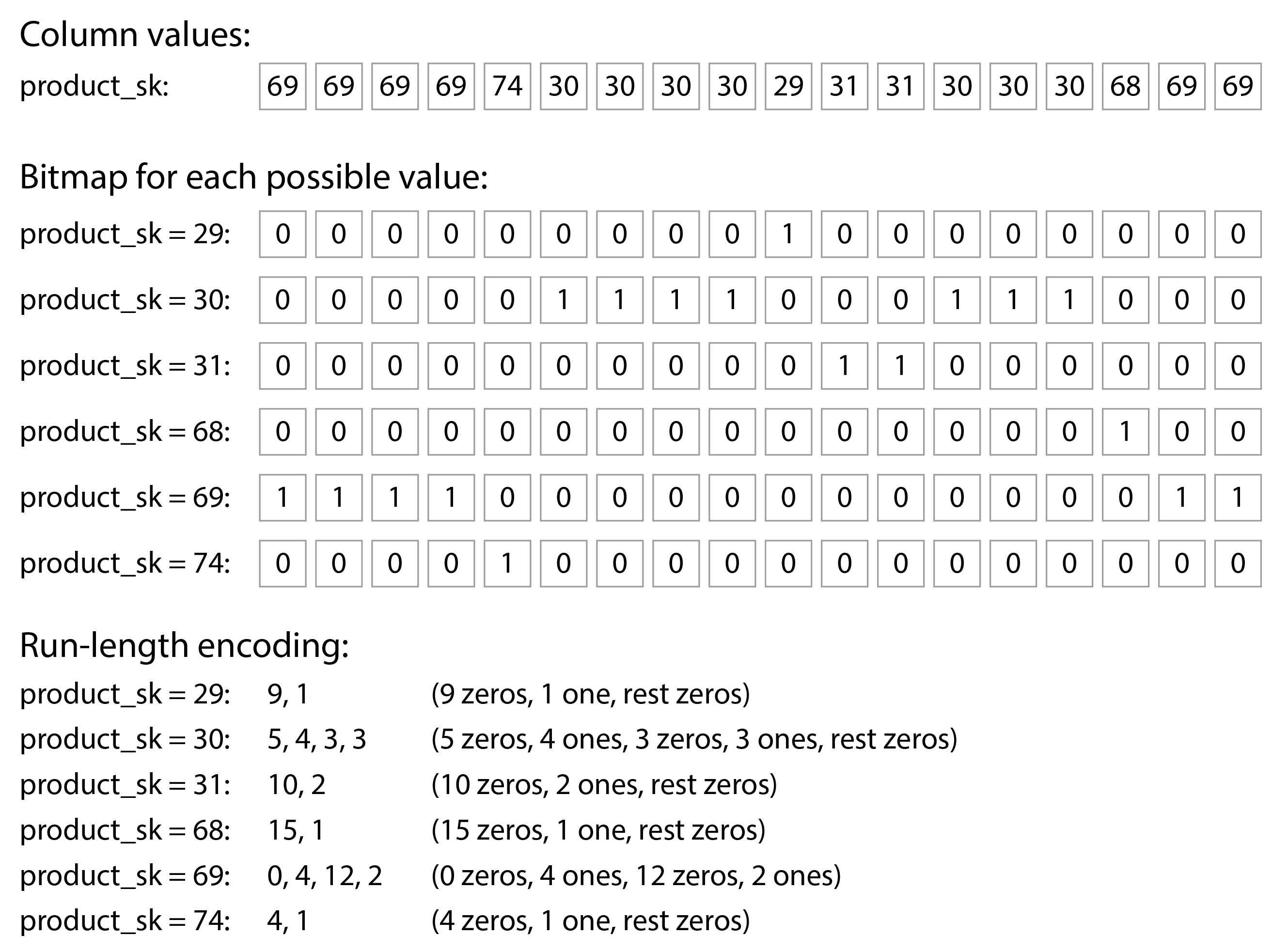
Columnar storage layout with bitmap and run-length encoding (RLE) compression.
To maximize efficiency, columnar databases typically employ a two-step compression strategy:
- Bitmap Encoding: Instead of storing raw, multi-byte values, the engine identifies each distinct value and creates a separate bit array (bitmap) for it. The array simply records
1if the value is present in that row and0if it is not (e.g.,[1, 1, 1, 1, 0, 0...]). This reduces the storage cost to a single bit per row. - Run-Length Encoding (RLE): Because sorted data produces long, contiguous streaks of identical bits, RLE compresses the bitmap further by merely recording the counts of consecutive 0s and 1s. Rather than storing a dozen
0s individually, RLE condenses it by recording the number12.
Combining Bitmap Encoding and RLE compresses billions of rows into a few kilobytes, significantly reducing I/O overhead and accelerating analytical queries.
(列式儲存具備高度壓縮潛力。系統透過「點陣圖編碼」轉換欄位值,再搭配「游程編碼 (RLE)」記錄連續相同值的數量,將海量資料壓縮至極小體積以節省 I/O 負擔。)
Sort Order in Column Storage
In columnar databases, columns cannot be sorted independently, as doing so would destroy the row alignment. Instead, the data must be sorted conceptually as entire rows based on a designated hierarchy of keys before being stored as individual columnar files.
- Primary Sort Key: Setting a primary sort key (e.g., Date) creates extended, contiguous sequences of identical values in that column, making run-length encoding (RLE) highly effective.
- Secondary Sort Keys: The compression benefits experience diminishing returns. A secondary key (e.g., Product) is only sorted within the localized, fragmented chunks established by the primary key. By the third or fourth key, the data order often appears randomized, offering minimal compression.
Despite this diminishing return, multi-level sorting remains a net win, as it accelerates highly localized queries and maximizes compression where it matters most.
(列式資料必須整行一起排序。設定第一排序鍵能產生極長的連續值,使 RLE 壓縮效益最大化;第二排序鍵以後的連續值會逐漸受限於前層邊界而碎片化,導致壓縮效益遞減。儘管如此,多重排序仍有助於加速局部查詢。)
Writing to Column-Oriented Storage
Inserting or modifying a single row directly into a compressed, sorted columnar file is highly inefficient. Inserting a new value in the middle requires rewriting the entire file to shift subsequent values and recalculate the compression—a significant overhead for a single update. To overcome this, modern column-oriented databases borrow the memory buffering concept from LSM-trees:
- Memory Buffering: New incoming writes are buffered in an in-memory store (often row-oriented for fast insertion) instead of touching the immutable on-disk files.
- Background Merge: Once the buffer reaches a threshold, a background process merges it with older on-disk columnar files to write a brand new, compressed segment.
- Read Merging: To return accurate results, the query engine must simultaneously scan the on-disk files and the uncompressed in-memory buffer, merging the results on the fly.
This architecture provides real-time query visibility while protecting the underlying disk from excessive write amplification.
(直接單筆寫入列式檔案成本過高,因需重寫全檔以維持壓縮。為此,系統導入記憶體緩衝機制:新資料先寫入記憶體,累積後再於背景批次寫入硬碟。查詢時則動態縫合兩者資料,確保結果即時性。)
Query Execution: Compilation and Vectorization
When scanning hundreds of millions of rows, traditional row-by-row query interpretation becomes a significant CPU bottleneck due to constant function-call overhead and poor branch prediction. To prevent this, modern data warehouses rely on two advanced optimization paradigms:
- Query Compilation: Instead of a generic interpreter loop, the engine generates and Just-In-Time (JIT) compiles custom, low-level machine code tailored specifically to the submitted SQL query. This strips away unnecessary conditional branches, executing logic at optimized speeds.
- Vectorized Processing: Instead of iterating row-by-row, the database processes contiguous batches (vectors) of columnar data simultaneously using CPU SIMD (Single Instruction, Multiple Data) instructions. The engine can execute highly efficient bitwise operations across bitmaps of 64+ rows in a single CPU cycle, often operating directly on compressed data.
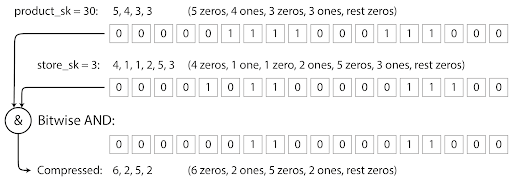
(為避免傳統逐列掃描造成 CPU 效能瓶頸,現代倉儲採用兩大最佳化策略:查詢編譯透過 JIT 技術即時生成專屬機器碼以消除直譯負擔;向量化處理則結合 CPU SIMD 指令,以批次方式平行運算點陣圖,顯著提升分析速度。)
Materialized Views and Data Cubes
To avoid repeatedly recomputing expensive aggregations over billions of rows, data warehouses use materialized views—query results physically saved to disk.
A specialized implementation is the Data Cube, a multi-dimensional grid (e.g., Date $\times$ Product). It pre-calculates aggregates for every intersection and margin total. Queries matching these exact dimensions are resolved instantly by reading a single pre-computed cell.
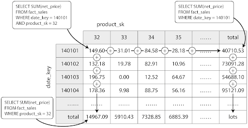
However, Data Cubes suffer from an inherent lack of flexibility. If a query filters on an attribute not built into the cube's dimensions (e.g., Price > $100$), the cube becomes ineffective. The database engine must bypass the cube and perform a resource-intensive full-table scan of the raw, un-aggregated data.
(為避免重複計算,系統利用物化檢視將聚合結果實體化。資料立方體是其多維度版本,能透過預先算出各維度總計來提供即時查詢。然而其缺乏彈性,若查詢條件超出預設維度,系統只能被迫回退至耗時的全表掃描。)
Multi-dimensional Indexes
Standard composite indexes act like a phonebook, requiring queries to proceed sequentially from left to right. They are ineffective for multi-dimensional spatial queries (e.g., finding data within a rectangular map area) because they would scan a broad latitudinal band before filtering for longitude. To resolve this, databases employ multi-dimensional indexes:
- Spatial Partitioning (e.g., R-Trees): Divides space into a hierarchy of overlapping bounding rectangles. Queries only drill down into rectangles intersecting the search box, eliminating irrelevant data.
- Space-Filling Curves: Mathematical techniques that map a 2D space into a 1D scalar value, allowing standard B-trees to store and query spatial data.
Multi-dimensional indexing applies beyond geography to any multi-range filtering. For instance, e-commerce platforms can index 3D RGB color values, or system logs can treat time and temperature (e.g., November 2025 and 10°C to 18°C) as a 2D coordinate system to efficiently isolate target records without a full scan.
(傳統聯合索引必須由左至右查詢,不利於二維空間檢索。資料庫對此採用多維索引:如 R 樹以邊界矩形排除無關區域,或以空間填充曲線將二維降維至一維存入 B 樹。此技術也適用於任何多重範圍過濾,如 RGB 顏色或特定氣溫與時間區間,將條件視為空間座標以精準定位資料,減少無效掃描。)
Full-Text Search and Fuzzy Matching
Conceptually, full-text search engines treat documents as a high-dimensional space where every possible word is a distinct dimension. They rely on an Inverted Index, mapping words to lists of document IDs. By converting these lists into bitmaps, engines resolve multi-word queries rapidly using hardware-accelerated bitwise operations.
To handle partial matches or typographical errors, engines employ algorithmic techniques:
- N-grams: Breaking words into overlapping fragments (e.g., "hello" into "hel", "ell", "llo") enables complex substring and regex searches, though it results in a larger index size.
- Tries and Edit Distance: To tolerate typos, tools like Lucene store vocabulary in memory using deterministic finite automatons (similar to a Trie). This allows the engine to traverse the structure and calculate the Levenshtein edit distance dynamically, retrieving closely matched terms without scanning the entire dictionary.
(全文搜尋引擎將文章視為高維度空間,透過倒排索引將單字對應至文章 ID 清單,並轉為點陣圖以利位元運算。為處理局部比對或拼字錯誤,系統可將單字切分為 n-gram 以支援正規表達式,或以類似 Trie 的樹狀結構儲存字典,藉由動態計算編輯距離以高效找出相近詞彙。)
Vector Embeddings and Semantic Search
Semantic search overcomes the limitations of exact keyword matching by understanding user intent. Machine learning models generate Vector Embeddings—high-dimensional coordinates representing the semantic meaning of data. Concepts with similar meanings are placed closer together, allowing engines to find relevance by calculating spatial distance.
To find the "nearest neighbors" across millions of vectors efficiently, databases use specialized indexes:
- Flat Index (Brute-Force): Computes the distance against every vector. It guarantees 100% accuracy but is computationally expensive ($O(N)$).
- Inverted File Index (IVF): Partitions the vector space into clusters. Searches only evaluate the nearest cluster's center point, trading some accuracy for significant performance improvements.
- HNSW (Hierarchical Navigable Small World): Functions like a multi-dimensional skip list across a multi-layered graph. The search makes large spatial leaps on sparse top layers, then drops to dense lower layers to pinpoint nearest neighbors, minimizing distance calculations.
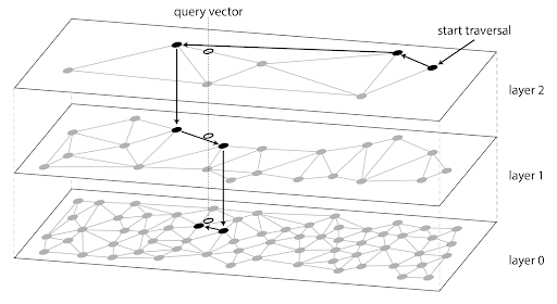
(語義搜尋透過機器學習模型將資料轉為高維度座標的「向量嵌入」,藉由空間距離來判斷語意相似度。為高效找出最近鄰居,資料庫採用專屬索引:如精準但運算成本高的平面索引、以分區聚類換取速度的 IVF,以及利用多層級圖論進行跳躍式搜尋的 HNSW,以克服高維度比對的效能瓶頸。)
Wrapping Up
To wrap up, understanding how databases store and retrieve data essentially boils down to understanding the target workload:
- OLTP (Operational Workloads): Designed for fast, point-in-time transactions. The architectural choice here is generally between B-trees, which offer predictable read performance through in-place updates, and LSM-trees, which maximize write throughput by converting random updates into sequential disk operations.
- OLAP (Analytical Workloads): Built to scan and aggregate massive datasets. These systems abandon row-oriented structures in favor of column-oriented storage, leveraging aggressive compression techniques (like Bitmaps and RLE) and vectorized CPU processing to bypass disk I/O bottlenecks.
- Multi-dimensional and Advanced Search: When standard 1D composite indexing is ineffective, databases turn to specialized structures. Whether utilizing R-trees for spatial boundaries, inverted indexes for full-text queries, or HNSW graphs for semantic vector embeddings, these indexes map complex, multi-dimensional conditions into efficient retrieval paths.
(總結來說,資料庫的底層設計取決於其工作負載:OLTP 系統專注高頻交易,透過 B 樹提供穩定的讀取,或以 LSM 樹換取極致的寫入吞吐量;OLAP 系統針對海量分析,改採列式儲存並高度依賴資料壓縮與向量化運算來突破 I/O 瓶頸;面對超越一維條件的複雜場景,則仰賴 R 樹、倒排索引或向量索引等特殊結構,將空間、全文或語意搜尋轉化為高效的檢索路徑。)


